Toy Problem
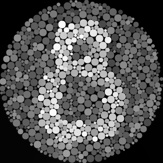
We need to reconstruct the following image from a system of linear equations:
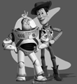
The purpose of this exercise was for me to get used to setting up a system of linear equations in the form of \(A \bf{v} = \bf{b}\).
There are 3 constraints that must be taken in consideration when building the system. Take notice I use notation of \((y, x)\) for the plane as opposed to \((x, y)\):
- Minimize \(((v(y, x + 1) - v(y, x)) - (s(y, x + 1) - s(y, x)))^2\)
- Minimize \(((v(y + 1, x) - v(y, x)) - (s(y + 1, x) - s(y, x)))^2\)
- Set \(v(0, 0) = s(0, 0)\)
We can think of \(\bf{v}\) as the pixels for the resulting image, and that is what we want to solve for in our system. \(\bf{b}\) then contains values of our knowns, and the matrix \(A\) is a sparse matrix consisting of all the terms in the form of \(v(y, x + 1) - v(y, x)\) or \(v(y + 1, x) - v(y, x)\). Finally, the source image is denoted as \(s\).
The last constraint of \(v(0, 0) = s(0, 0)\) helps with adding a known pixel value into the system which will then cause the system to be solved with values in \(\bf{v}\) close to that of the original image. This essentially makes the variable associated with \(v(0,0)\) within \(\bf{v}\) to be known and thus used for the entire system.
$$ A\bf{v} = \begin{bmatrix} -1 & 1 & 0 & ... & ... & ... & ... & ... & 0 \\ 0 & -1 & 1 & ... & ... & ... & ... & ... & 0 \\ ... \\ 0 & ... & -1 & ... 1 & ... & ... & ... & ... & 0 \\ 0 & ... & 0 & ... & -1 & ... & 1 & ... & 0 \\ ... \\ 1 & 0 & 0 & ... & ... & ... & ... & ... & 0 \\ \end{bmatrix} \begin{bmatrix} v_{0, 0} \\ v_{0, 1} \\ ... \\ v_{1, 0} \\ v_{1, 1} \\ ... \\ v_{nr \times nc} \end{bmatrix} = \begin{bmatrix} s(0, 1) - s(0, 0) \\ s(0, 2) - s(0, 1) \\ ... \\ s(1, 0) - s(0, 0) \\ s(2, 0) - s(1, 0) \\ ... \\ s(0, 0) \end{bmatrix} $$
Once \(\bf{v}\) is solved, we can build the image out of the elements within the column vector. The comparison between the original image and reconstructed image is shown below:
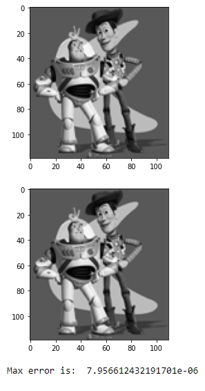
The maximum error between each pixel should be minimal. In my specific implementation, I was able to achieve a maximum error of \(7.9566 \times 10^{-6}\). The acceptable error should be less than \(1.0 \times 10^{-3}\)
Poisson Blending
Once setting up the system of linear equations is understood, Poisson Blending can be less intimidating.
The algorithm assumes two images as input:
- The source image \(s\) which will be used as the object to be pasted onto some background image.
- The target image \(t\) which is the background image that the source image will be pasted onto.
There are two blending constraints that the system must adhere to when solving \(A\bf{v} = \bf{b}\).

Let's try to dissect the expression. The first term of the constraint takes in a pixel \(i\) which is in the current location \((y, x)\) in the source image, \(S\). Then for each pixel \(j\) within the 4-connected neighborhood \(N_i\) of \(i\) within the source image, we must minimize the error in between these pixels for \(i\).
This leads us to having 4 equations to solve for every pixel \(i\) not considering boundaries.
The second constraint takes in a pixel \(i\) at every location \((y, x)\) in the source image, \(S\). Then for every pixel \(j\) in the 4-connected neighborhood \(N_i\), we must only take pixels which fall outside of the source image along with the corresponding location of \(j\) within the background image.
The second constraint also leads us to having 4 equations to solve for every pixel \(i\) not considering boundaries.
Once all pixels in \(\bf{v}\) have been solved, we copy the pixels over into the location at the background image to create a final blended image.
Example 1
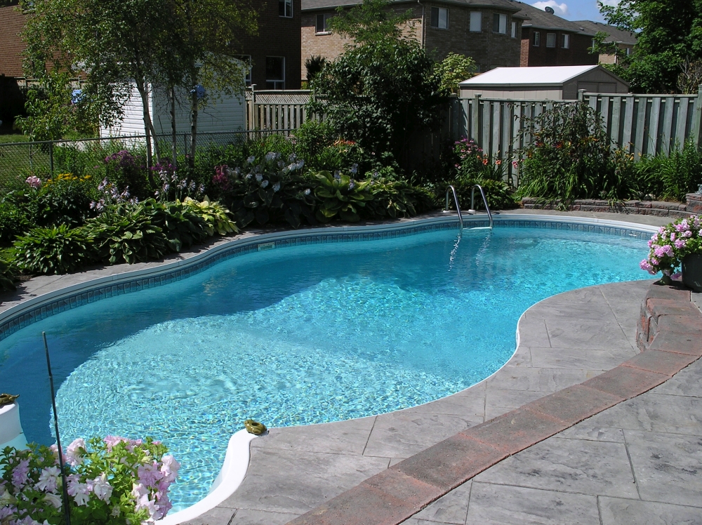
This is personally my favorite example. I used an image of a pool (background image) and a 3D render of Squirtle (object image) and created a final blended image of Squirtle standing in front of the pool ready to take a nice swim.
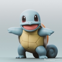
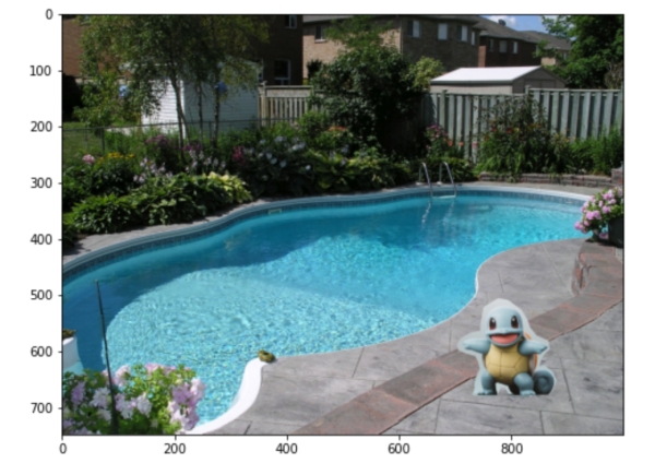
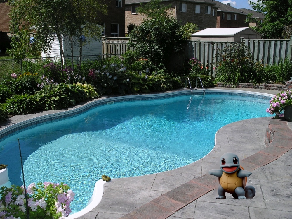
Notice that to minimize the error between pixels, the color of Squirtle changes slightly to match the tone of the pool's concrete. This result tells us that it is best to choose an object that will be pasted onto the background image with an overall color tone that is similar to the background image to minimize the shift in colors.
Example 2
I had fun with this one as a father. We have all been there where our small children, or infants terrorizing our lives. For me, I have had a bit of PTSD hearing a baby cry as a result from lack of sleep during the nights when my daughter was a newborn. To pay some tribute to those days, I decided to blend her face into a cup of coffee. 😂

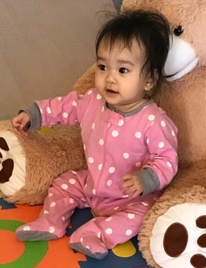
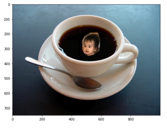
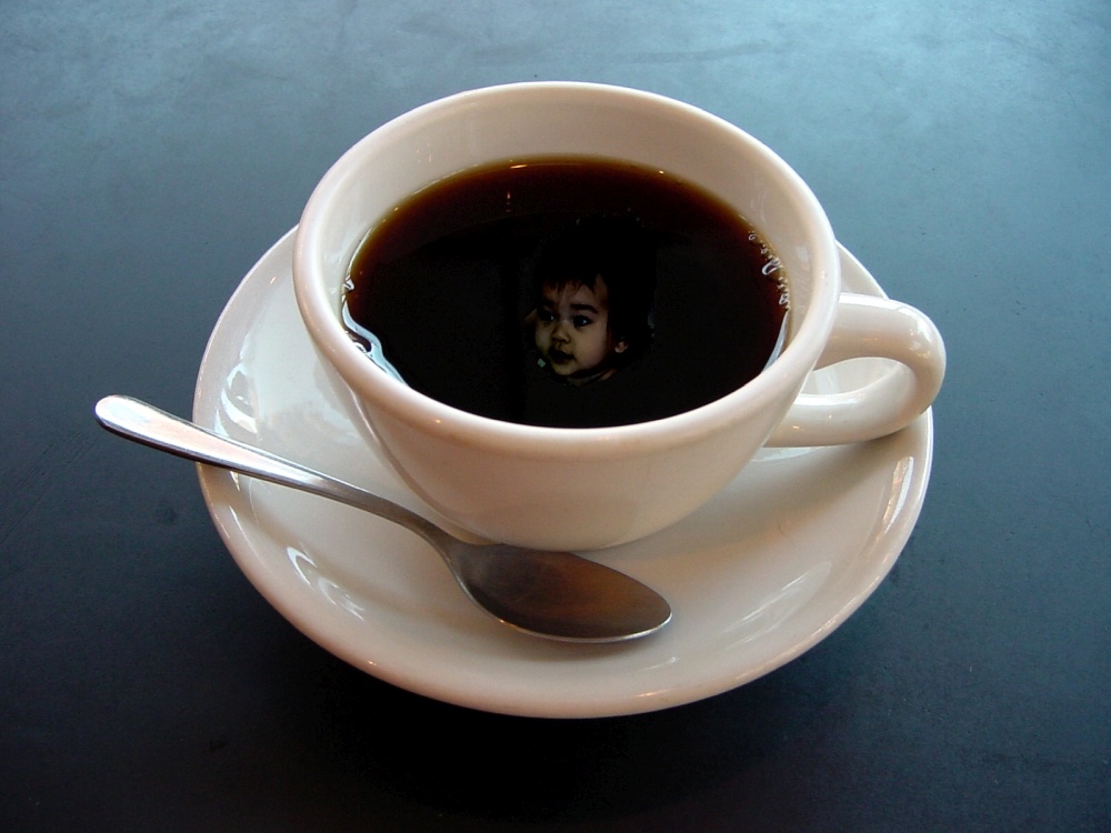
The shift in tone of Riley's face to a darker one to match that of the coffee cup is perfect for the effect I wanted to give for this picture. Notice again, that it is the object image that changes color when being blended into the background. I wanted to give the haunting feeling to how much a baby can bring someone to their knees. 😁 Thus having a faded blend was perfect. If I did not want this shift in tone, I would have probably used a lighter color liquid as the background picture.
Failed Example
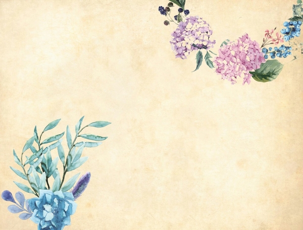
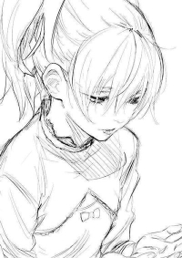
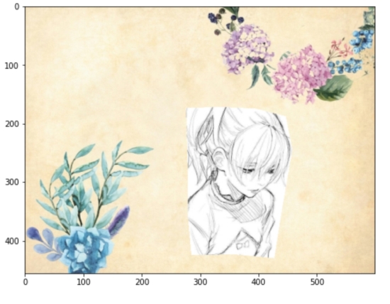
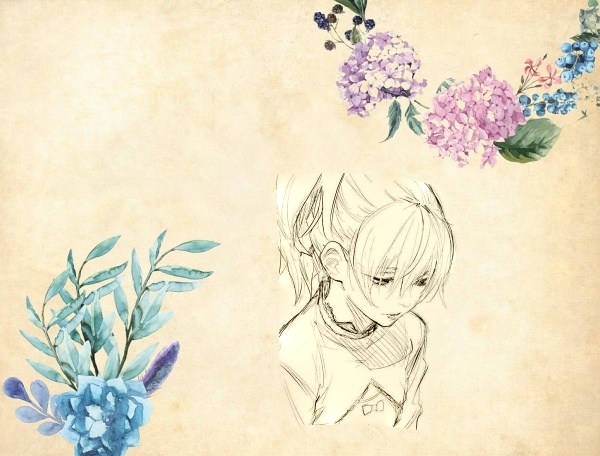
I attempted to blend a sketch onto stationary. I consider this to be a failed example because even after Poisson Blending, the sketch on stationary does not look convincing at all. The viewer will still be able to tell that it could be a bad copy, and paste job onto the stationary. The background area of the sketch has changed color, but still does not have the same texture and tone as the stationary.
I suspect that this example failed because of the sketch being an image with a lot of high frequency data with all the lines being pasted onto an image with low frequency where there is not much data aside from the flowers.
Mixed Gradient
This is a modification to Poisson Blending. As stated in the project instructions, this time the expressions look like:

With this approach, there is still the same number of equations needed to evaluate the image. However the constraints are modified like so:
- We do not directly use the source gradient against current pixels and its neighborhood. Instead, we use the larger gradient magnitude between either the source pixel's neighborhood, or the target image pixel that falls within the corresponding source pixel's neighborhood.
- We add the target image pixels that is within the corresponding source pixel's neighorhood, but not within the source image itself with the larger gradient magnitude like the first (1) constraint.
Example 1
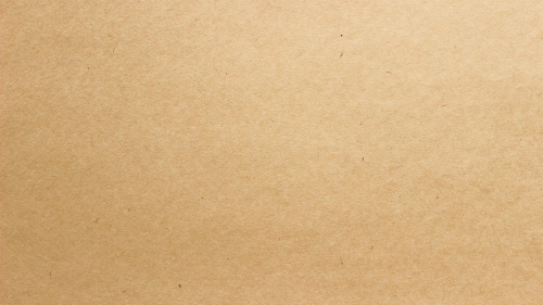
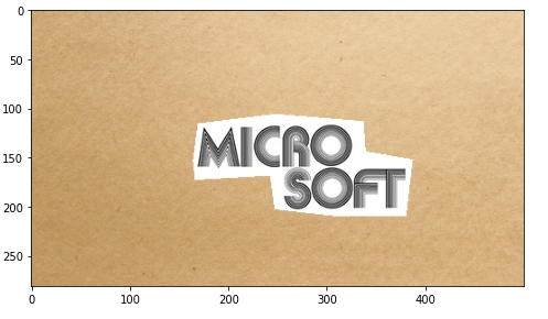
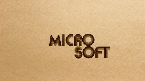
Here is an example of blending text onto a plain surface. For the plain surface, I have decided to use an image of paper.
For the object image to be pasted onto paper, I decided to use the vintage logo of my employer. Maybe something similar will be printed and go for sale in the company store...

Example 2
Going back to the stationary example, I wondered what an image would look like if it was pasted on this type of texture?
This time I decided to use a picture of a jellyfish.
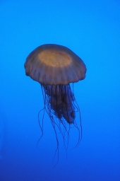
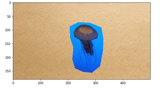
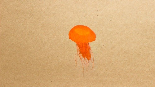
I think the result is visually pleasing. It could be a good wallpaper if the image is at a higher resolution.
Color2Gray
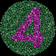
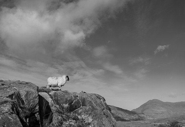
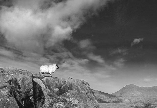
The task here is to be able to maintain some of the details that may be lost when converting an RGB image to grayscale. This is like the Toy Problem, but with mixed gradient approach.
The approach here is to find the largest gradient magnitude so that the changes will be more prominent. We will use the channel with the largest gradient magnitdue as the target image for guidance.
Once we find the channel to be used, we will then go through each channel of the input RGB image and apply the mixed gradient approach. For every pixel, we use either the gradient from the source, or the target -- whichever is greater.
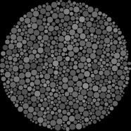
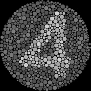
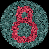
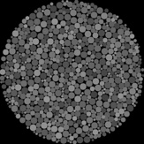
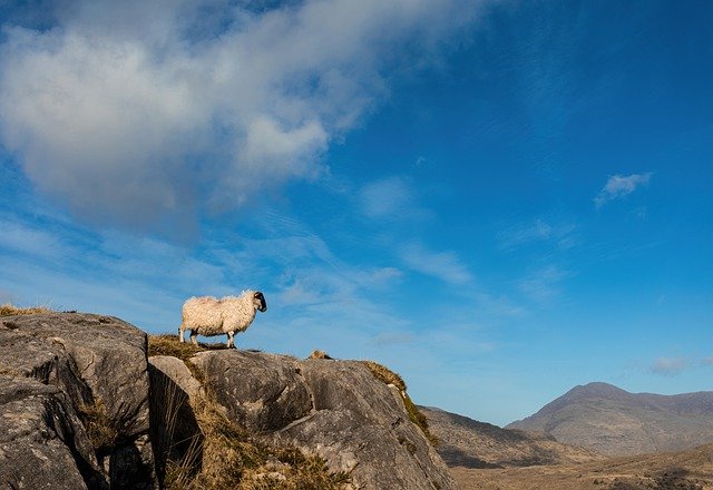
The following results are shown for 2 color blind test images, and 1 natural image.
Laplacian Blending
We would like to compare the results in pasting an object onto an image and blending using Laplacian Blending as opposed to Poisson Blending.
To properly blend an image using Laplacian Blending, we must construct 3 pyramids:
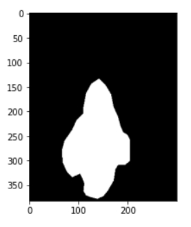
- Alpha Matte - The Gaussian Pyramid with the combined mask of the object image mask pasted onto the target
- Source Pyramid - The Laplacian Pyramid of the source image (the object to be pasted)
- Target Pyramid - The Laplacian Pyramid of the target image (the background image for object to be pasted onto)
In my implementation, I had decided to use a pyramid size of 4, consisting of images of 1x, 2x, 4x, and 8x downsampling factors.
For each level \(i\), we want to apply the following formula to construct a new pyramid of the combined images:
$$ R_{i} = \alpha_{i} * Ls_{i} + (1 - \alpha_{i}) * Lt_{i} $$
Where \(\alpha\) is the current Gaussian mask to be applied onto the Laplacian images of the source and target.
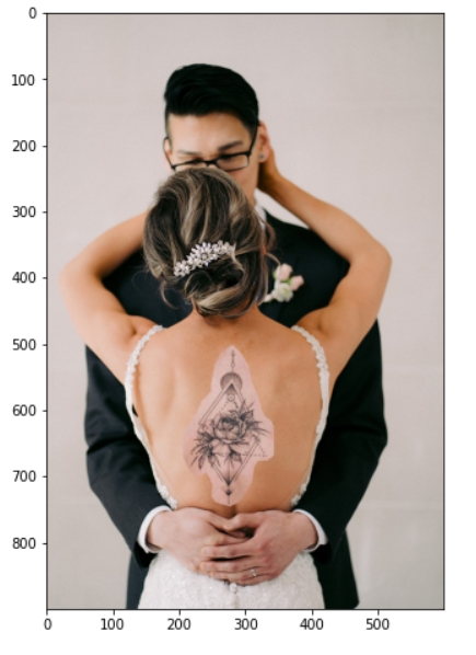
Once build the new pyramid with combined images, \(R\), we can then collapse the pyramid by adding all images within the combined pyramid to achieve the final blended image.
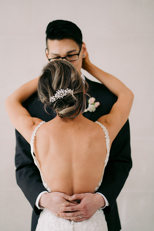
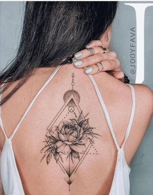
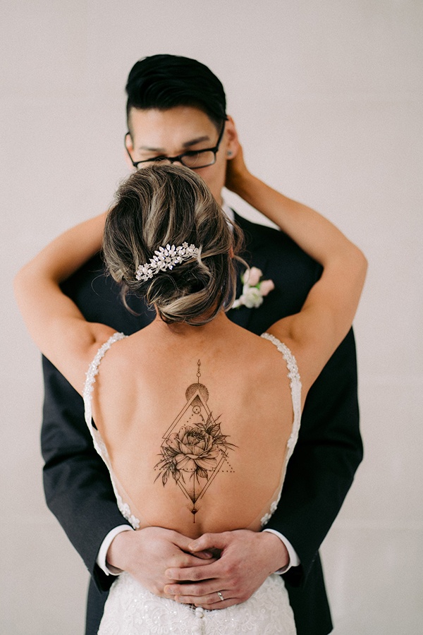
Example
I chose to use one of my wedding photos as a background image and a picture of a woman's back with tattoo as the object image. For the final blended result, I want to be able to achieve the effect of giving my wife a tattoo.


Sharpen Filter using Gradients
We can also use Gradient Domain editing to create image filters that can accentuate the edges of the image to sharpen them. The approach I decided to achieve this is to increase the gradient values by multiplying the gradients of each pixel by some \(\alpha\) constant within the image \(S\).
My approach also involves increasing the gradients in both the horizontal, and vertical directions. There are 3 constraints:
$$ \alpha(s(y, x + 1) - s (y , x)) = t(y, x + 1) - t (y, x) $$
$$ \alpha(s(y + 1, x) - s (y , x)) = t(y + 1, x) - t (y, x) $$
$$ s(y, x) = t(y, x) $$
The first two will attempt to increase the gradient values while the last constraint maintains the color of the image.
The following picture was taken from a attriburted source, and subsequently blurred to exaggerate the comparison between a blurry image and the sharpened image utilizing gradient domain editing.

Acknowledgements and Attributions
- Swimming Pool - https://en.wikipedia.org/wiki/Swimming_pool
- Squirtle - https://www.myminifactory.com/object/3d-print-squirtle-pokemon-137107
- Coffee Cup - https://indianapublicmedia.org/amomentofscience/coffee-cup-convection.php
- Flower Stationary - https://pixabay.com/illustrations/flower-background-floral-vintage-3307894/
- Sketch - https://www.deviantart.com/yousofashraf/art/549962-589933007684213-1310625107-N-390192853
- Paper Stationary - https://pixabay.com/photos/paper-texture-brown-natural-1468883/
- Vintage Microsoft Logo - https://logovector.net/tag/microsoft
- Jellyfish (Paul Brennan) - https://pixabay.com/photos/jelly-fish-sting-aquatic-sea-1911686/
- Sheep on Mountain (Jon Pauling) - https://pixabay.com/photos/sheep-mountains-rural-ireland-5929158/
- Back Tattoo - https://www.pinterest.com/pin/263531015685875275/
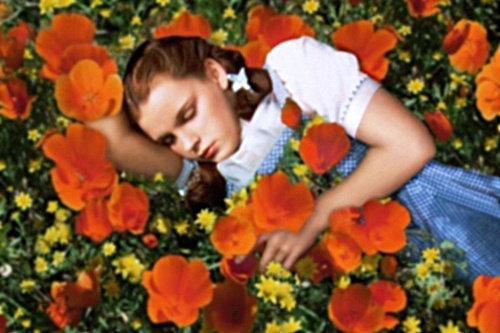
- Judy Garland - https://www.anothermag.com/art-photography/2716/top-10-flowers-on-film-moments
Last modified: February 2021, Roger Ngo, urbanspr1nter@gmail.com